Exploring 2D differentiable rendering
Going in depth on how 2D differentiable rendering/rasterization works and reimplementing it using PyTorch.
Experimenting with differentiable rendering
Introduction
In its most fundamental form, the core idea behind differentiable rendering (DR) is to reformulate/approximate the rendering function so that the output pixels are continuous and smooth (differentiable) with respect to the input parameters (which can be 3D/2D geometry, lighting conditions, material properties, camera positioning, etc).
Now, by itself, differentiable rendering won't solve all problems depending on what your input represents; for instance, if you're solving for 2D geometry and a shape is on top of another shape, the optimizer will have basically no knowledge of the shape underneath since it's not affecting anything in the output image (thus you get zero gradients for the shape underneath). While this is a fundamental limitation of 2D rendering, there are fixes for such issues (e.g., enforcing a small baseline transparency or soft opacity prior).
Signed distance functions (SDFs)
SDFs play a huge part in 2D differentiable rendering (and I'd guess 3D DR too), so we first have to understand how they work.
In principle, SDFs are really simple: we just want to define a function that, given x, y, and whatever other parameters your primitive needs (e.g., Px, Py, Pradius for a circle), it returns a new z value.
If this z value is positive (>0), then we're inside the primitive; otherwise, if it is negative (<0), we're outside the primitive (hence the signed in the name).
Important
Sign conventions change across the literature.
What I will be using here (positive inside, negative outside) is perfectly valid. But most adopt the opposite (negative inside, positive outside).
The boundary is always at , so this choice doesn't affect the output. It just flips the gradient direction during optimization.
It is definitely something to be aware of, though.
For example, to define a circle, we can use the following:
Where are our current grid position, are the position of our circle, and is the radius of our circle.
Here we are literally just measuring the distance (the function) to a point and adding a threshold () to make a circle.
Obviously, we can also negate the function (which would be ) so that negative is inside the shape and positive is outside.
Now, if we graph it, we get the following:
Now, notice how, when the function isn't normalized, it defines a gradient in which the sign indicates whether we are inside or outside the shape.
You'll also notice the undulating stripes in the visualization; those are the sine of the function output ().
They don't have a specific use in our case, but they do visually encode the gradient field, making it easier to see how the SDF changes smoothly across space.
Of course, we will lose the full gradients when we squish the function by normalizing it, but the gradients will live within the slope of that normalization function.
Obviously, we aren't limited to just circles; we can make basically any primitive, or make them intersect, unify, subtract, and so much more.
For instance:
| Operation | Function (>0 in, <0 out) | Function (<0 in, >0 out) |
|---|---|---|
| Union | ||
| Intersection | ||
| Subtraction |
Where are two SDFs
Tip
SDFs in PyTorch
Note
Before we begin this section, note that the Python Notebook for this is available here.
Just in case you're like me and would much rather read code over yapping.
Defining the grid
Much like in GPUs, where each pixel is evaluated in parallel, the exact same can be done in PyTorch.
So we can begin by defining a grid with size (width, height) in the range (0 to (width - 1), 0 to (height - 1)), like so:
import torch
import torch.nn as nn
import matplotlib.pyplot as plt

def plot_output(ax, value, title = None, **kwargs):
    ax.imshow(value.detach().cpu().numpy(), **kwargs)
    if title: ax.set_title(title)
    ax.axis("off")

grid_size = (64, 64)

grid_x_vals, grid_y_vals = [torch.arange(sz, dtype=torch.float32) for sz in grid_size]
grid_y, grid_x = torch.meshgrid(grid_x_vals, grid_y_vals, indexing="ij")

fig, axes = plt.subplots(1, 3, figsize=(12, 3 * 2.6))

plot_output(axes[0], grid_x, f"Grid X")
plot_output(axes[1], grid_y, f"Grid Y")

def normalize(t):
    t_min, t_max = t.min(), t.max()
    return (t - t_min) / (t_max - t_min + 1e-8)

red = normalize(grid_x)
green = normalize(grid_y)
blue = torch.zeros_like(red)

plot_output(axes[2], torch.stack([red, green, blue], axis=-1), f"Grid X and Y")

fig.tight_layout()
plt.tight_layout()
plt.show()
plt.close()
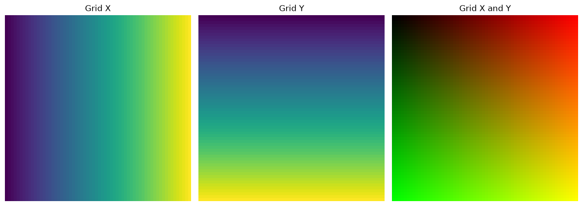
This gives us the following:
Applying an SDF function to it
Now we can simply apply an SDF function to each one of those values (much like how you would do in a GPU shader).
So using the following code:
pos_x = 32.0
pos_y = 32.0
radius = 8.0

def sdf_circle(grid_x: torch.Tensor, grid_y: torch.Tensor, pos_x, pos_y, radius):
  return radius - torch.sqrt((grid_x - pos_x + 1e-4) ** 2 + (grid_y - pos_y + 1e-4) ** 2)

def smoothstep(edge0: torch.Tensor, edge1: torch.Tensor, x: torch.Tensor) -> torch.Tensor:
  t = torch.clamp((x - edge0) / (edge1 - edge0 + 1e-4), 0.0, 1.0)
  return t * t * (3.0 - 2.0 * t)

def norm_atan(sdf): return torch.atan(sdf) / torch.pi + 0.5
def norm_atanx4(sdf): return torch.atan(sdf * 4) / torch.pi + 0.5
def norm_tanh(sdf): return torch.tanh(sdf) / 2 + 0.5
def norm_sigmoid(sdf): return torch.sigmoid(sdf)
def norm_smoothstep(sdf): return smoothstep(-0.5, 0.5, sdf)

sdf_raw = sdf_circle(grid_x, grid_y, pos_x, pos_y, radius)
sdf_atan = norm_atan(sdf_raw)
sdf_atanx4 = norm_atanx4(sdf_raw)
sdf_tanh = norm_tanh(sdf_raw)
sdf_sigmoid = norm_sigmoid(sdf_raw)
sdf_smoothstep = norm_smoothstep(sdf_raw)

fig, axes = plt.subplots(1, 6, figsize=(16, 6))

def plot_sdf_normalizations(axes):
  plot_output(axes[0], sdf_raw, f"Circle SDF (raw)", vmin=0, vmax=1)
  plot_output(axes[1], sdf_atan, f"Circle SDF (atan)", vmin=0, vmax=1)
  plot_output(axes[2], sdf_atanx4, f"Circle SDF (atanx4)", vmin=0, vmax=1)
  plot_output(axes[3], sdf_tanh, f"Circle SDF (tanh)", vmin=0, vmax=1)
  plot_output(axes[4], sdf_sigmoid, f"Circle SDF (sigmoid)", vmin=0, vmax=1)
  plot_output(axes[5], sdf_smoothstep, f"Circle SDF (smoothstep)", vmin=0, vmax=1)

plot_sdf_normalizations(axes)

fig.tight_layout()
plt.tight_layout()
plt.show()
plt.close()
This pretty much just evaluates the SDF for every point in our grid, so we're feeding that entire 64x64 grid to the SDF; the SDF calculates a new value (our ) for every point and returns a new 64x64 grid.
We get the following:

I don't think I need to mention this; you are not limited to these functions. You can use practically any normalization function (keep in mind it might change how things work drastically even if visually it looks the same; we will see this happening in action later on).
Creating a simple target image
So we have to define a target to optimize for; let's begin by just using a circle (which can be defined by our own circle SDF).
target = sdf_circle(grid_x, grid_y, pos_x * 1.5, pos_y * 1.5, radius).clamp(-1, 1) / 2 + 0.5
fig, axes = plt.subplots(1, 1, figsize=(2.6, 2.6))

plot_output(axes, target, f"Image target", vmin=0, vmax=1)

fig.tight_layout()
plt.tight_layout()
plt.show()
plt.close()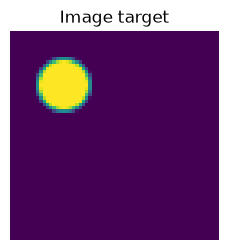
Visualizing the function gradients
Now, before our first training run, I think it would be neat to see how the gradients vary across the functions.
The good thing about circles is that we only have 3 parameters that we can touch (, , ), thus we can lock and create a 2D vector field to see how the gradients will flow.
So how do we do that? Well, it's actually quite straightforward:
- The gradient is basically back-propagation telling us how we should change our parameters (so it's a delta). Thus, we start by defining a tensor that stores that delta (same size as the number of parameters), for every sample we want to get and for every type of function we have (which is 6:
raw,atan,atanx4,tanh,sigmoid,smoothstep). We do the same with loss, but loss is represented by a single number. - We iterate over every point we would like to sample and track its index (we have to know which sample the current gradient vector and loss belong to).
- We define our parameters for the current sample. In this case, it is the current circle position (so and ).
- We compute
sdf_rawand then every other function type. - Now things get interesting because we call
write_grad. The first arguments are just info about which sample we're solving for, then the resulting value from our function, and finally the parameters we want to get the gradients for. - Inside
write_gradwe calculate the L2 loss and get the gradients usingtorch.autograd.grad. This function is very interesting because it only differentiates for parameters we manually gave it (theparamsvariable, so and ), it then returns the gradients as a list of tensors. At no point do we have to deal with hidden states,.grad.zero_(), or anything else. We also have to useretain_graph = Trueotherwise, PyTorch would free the compute graph after the firsttorch.autograd.gradcall. - We then store those values and graph them.
I won't get into the graphing part because it's really just about negating the gradients (by default the gradients go up; we want to go down), scaling them, and plotting them.
# [types, grid_x, grid_y, parameters]
vector_field = torch.empty((6, *grid_size, 2))
# [types, grid_x, grid_y, 1]
loss_field = torch.empty((6, *grid_size, 1))

def write_grad(idx: int, gx_idx: int, gy_idx: int, sdf: torch.Tensor, params: list[torch.Tensor]):
  loss_l2 = nn.functional.mse_loss(sdf, target)
  gradients = torch.autograd.grad(loss_l2, params, retain_graph=True, allow_unused=True)
  vector_field[idx, gx_idx, gy_idx] = torch.tensor(gradients, dtype=torch.float)
  loss_field[idx, gx_idx, gy_idx] = loss_l2.detach().clone()

for gx_idx in range(grid_size[0]):
  for gy_idx in range(grid_size[1]):
    gx_val = grid_x[gx_idx, gy_idx].detach().clone().requires_grad_(True)
    gy_val = grid_y[gx_idx, gy_idx].detach().clone().requires_grad_(True)

    sdf_raw = sdf_circle(grid_x, grid_y, gx_val, gy_val, radius)
    sdf_atan = norm_atan(sdf_raw)
    sdf_atanx4 = norm_atanx4(sdf_raw)
    sdf_tanh = norm_tanh(sdf_raw)
    sdf_sigmoid = norm_sigmoid(sdf_raw)
    sdf_smoothstep = norm_smoothstep(sdf_raw)

    write_grad(0, gx_idx, gy_idx, sdf_raw, [gx_val, gy_val])
    write_grad(1, gx_idx, gy_idx, sdf_atan, [gx_val, gy_val])
    write_grad(2, gx_idx, gy_idx, sdf_atanx4, [gx_val, gy_val])
    write_grad(3, gx_idx, gy_idx, sdf_tanh, [gx_val, gy_val])
    write_grad(4, gx_idx, gy_idx, sdf_sigmoid, [gx_val, gy_val])
    write_grad(5, gx_idx, gy_idx, sdf_smoothstep, [gx_val, gy_val])

sdf_titles = ["raw", "atan", "atanx4", "tanh", "sigmoid", "smoothstep"]
fig, axes = plt.subplots(2, len(sdf_titles), figsize=(15 * len(sdf_titles), 6 * 4))

def plot_grad_quiver(ax, grid_x, grid_y, plot_x, plot_y, color, title, scale):
  ax.pcolormesh(grid_x, grid_y, color, cmap="viridis", shading="auto", alpha=1)
  ax.quiver(grid_x, grid_y, plot_x, -plot_y, color, cmap="grey", scale=scale, alpha=1)
  ax.set_xlabel("x")
  ax.set_ylabel("y")
  ax.set_title(title)
  ax.grid(alpha=0.3)
  ax.set_aspect("equal", adjustable="box")
  ax.invert_yaxis()

def plot_grad_stream(ax, grid_x, grid_y, plot_x, plot_y, color, title, scale):
  grid_x_np = grid_x.detach().cpu().numpy() if torch.is_tensor(grid_x) else grid_x
  grid_y_np = grid_y.detach().cpu().numpy() if torch.is_tensor(grid_y) else grid_y
  plot_x_np = plot_x.detach().cpu().numpy() if torch.is_tensor(plot_x) else plot_x
  plot_y_np = plot_y.detach().cpu().numpy() if torch.is_tensor(plot_y) else plot_y
  color_np = color.detach().cpu().numpy() if torch.is_tensor(color) else color

  ax.streamplot(grid_x_np, grid_y_np, plot_x_np, plot_y_np, color=color_np, cmap="viridis", density=2, num_arrows=16, broken_streamlines=False)
  ax.set_xlabel("x")
  ax.set_ylabel("y")
  ax.set_title(title)
  ax.grid(alpha=0.3)
  ax.set_aspect("equal", adjustable="box")
  ax.invert_yaxis()

for idx, name in enumerate(sdf_titles):
  vx = vector_field[idx, :, :, 0]
  vy = vector_field[idx, :, :, 1]

  magnitude = torch.sqrt(vx ** 2 + vy ** 2)
  vx_normalized = torch.where(magnitude <= 1e-6, torch.tensor(0.0), vx / magnitude)
  vy_normalized = torch.where(magnitude <= 1e-6, torch.tensor(0.0), vy / magnitude)

  fixed_display_length = 0.05
  vx_plot = fixed_display_length * vx_normalized
  vy_plot = fixed_display_length * vy_normalized
  color = loss_field[idx, :, :].squeeze(-1)

  plot_grad_stream(axes[0, idx], grid_x, grid_y, -vx, -vy, color, f"Stream gradient ({name})", scale=0.25)
  plot_grad_quiver(axes[1, idx], grid_x, grid_y, -vx_plot, -vy_plot, color, f"Quiver gradient ({name})", scale=1.50)

fig.tight_layout()
plt.show()
plt.close()
This gives us the following graph (feel free to zoom in):
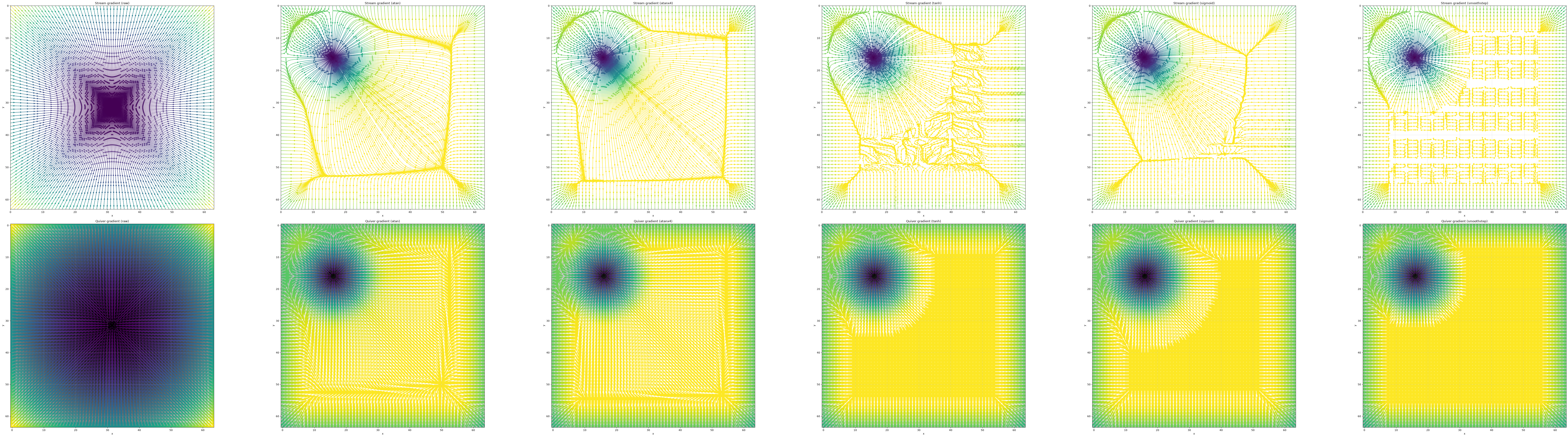
Now, even with just this graph, we can see some very interesting things and possible issues.
What I would like to point out is:
- How, with the raw non-normalized SDF, we get a direct unscaled gradient to the target, which is way stronger than with normalization. This makes sense, because the value that our SDF returns represents the distance to 0. Obviously, since our optimization target doesn't operate in the same range as the SDF (the numerical range for our target is 0 to 1, while SDFs don't have a singular range), the solution with the lowest loss is to set the circle in the middle.
- All functions give us valid gradients only around their optimization range, except
atanandatanx4which provide decent gradients for a bigger range than the others (which makes sense since it decays slowly). - How the truly meaningful gradients are close to the optimization target.
Now even with these issues, these functions will probably all perform relatively well because they produce a small area around them with decent gradients. While this would be a deal breaker basically anywhere else in ML, in this scenario we don't actually need fully continuous gradients, because having the optimizer trying to optimize every shape for the entire image is unnecessary. This way, the optimizer will try to fit shapes to their closest pixel.
We will actually see this exact issue of the optimizer being "too greedy" happening with atan and atanx4 later on.
First test runs
So now we can move to our first test runs.
For that I wrote this test bench:
import os, subprocess
from PIL import Image
from tqdm import tqdm

def convert_figure(fig):
  fig.canvas.draw()
  buffer = fig.canvas.buffer_rgba()
  sx, sy = fig.canvas.get_width_height()

  return Image.frombuffer("RGBA", (sx, sy), buffer, "raw", "RGBA", 0, 1)

def perform_combination_test(
  perform_run_fn,
  definition_list,
  definition_names,
  combination_list,
):
  for test_list_idx, test_case in enumerate(combination_list):
    test_enable = test_case["enable"]
    test_steps = test_case["steps"]
    test_name = test_case["name"]
    test_list = test_case["tests"]
    test_count = len(test_list)
    test_samples = []

    format_frame = "ppm"
    format_final = "webp"

    if not test_enable:
      continue

    for item in test_list:
      kw_args = {definition_names[idx]: definition_list[idx][key] for idx, key in enumerate(item)}
      samples = perform_run_fn(**kw_args, steps = test_steps)

      test_samples.append(samples)

    for sample_batch in tqdm(zip(*test_samples)):
      fig, axes = plt.subplots(2, test_count, figsize=(3 * test_count, 2.6 * 2))

      for test_idx, (step, sdf_norm, sdf_target, loss) in enumerate(sample_batch):
        run_setup = ", ".join(test_list[test_idx])
        plot_output(axes[0, test_idx], sdf_norm, f"{run_setup}\n[{step}] Loss: {loss:.6f}\nApprox", vmin=0, vmax=1)
        plot_output(axes[1, test_idx], sdf_norm - sdf_target, "Difference", vmin=-1, vmax=1)
        del sdf_norm

      fig.tight_layout()
      plt.tight_layout()
      convert_figure(fig).save(f"{test_name}.{step}.{format_frame}")
      plt.close()

    ffmpeg_cmd = f"ffmpeg -i '{test_name}.%d.{format_frame}' -framerate 25 -c:v libwebp -loop 0 {test_name}.{format_final} -y"
    print(subprocess.getoutput(ffmpeg_cmd))

    for idx in range(test_steps):
      os.remove(f"{test_name}.{idx}.{format_frame}")

norm_table = {
  "smoothstep": norm_smoothstep,
  "atan": norm_atan,
  "atanx1.5": lambda sdf: torch.atan(sdf * 1.5) / torch.pi + 0.5,
  "atanx2": lambda sdf: torch.atan(sdf * 2) / torch.pi + 0.5,
  "atanx3": lambda sdf: torch.atan(sdf * 3) / torch.pi + 0.5,
  "atanx4": norm_atanx4,
  "tanh": norm_tanh,
  "sigmoid": norm_sigmoid,
}
optimizer_table = {
  "rmsprop": (torch.optim.RMSprop, { "lr": 0.1, "momentum": 0.5 }),
  "adam": (torch.optim.Adam, { "lr": 2.0, "betas": (0.95, 0.999) }),
  "adamw": (torch.optim.AdamW, { "lr": 2.0, "betas": (0.95, 0.999) }),
}
circle_init_table = {
  "centered": (30.0, 30.0, 8.0),
  "offset": (48.0, 48.0, 8.0),
}

def perform_circle_run(norm_setup, optim_setup, vars_setup, steps):
  print(norm_setup, optim_setup, vars_setup, steps)
  px_init, py_init, rad_init = vars_setup
  p_x = nn.Parameter(torch.tensor(px_init))
  p_y = nn.Parameter(torch.tensor(py_init))
  p_radius = nn.Parameter(torch.tensor(rad_init))

  optim_module, optim_params = optim_setup

  optimizer = optim_module([p_x, p_y, p_radius], **optim_params)

  for step in range(steps):
    optimizer.zero_grad()
    p_radius.data.clamp_(1, 64)
    sdf_raw = sdf_circle(grid_x, grid_y, p_x, p_y, p_radius)
    sdf_norm = norm_setup(sdf_raw)
    loss = nn.functional.mse_loss(sdf_norm, target)

    loss.backward()
    optimizer.step()

    yield (step, sdf_norm.detach().clone().cpu(), target, loss.item())

perform_combination_test(
  perform_circle_run,
  [norm_table, optimizer_table, circle_init_table],
  ["norm_setup", "optim_setup", "vars_setup"],
  [
    dict(
      enable = True, steps = 200,
      name = "test-run-centered-rmsprop",
      tests = [
        ("smoothstep", "rmsprop", "centered"),
        ("atan", "rmsprop", "centered"),
        ("atanx4", "rmsprop", "centered"),
        ("tanh", "rmsprop", "centered"),
        ("sigmoid", "rmsprop", "centered"),
      ]
    ),
    dict(
      enable = True, steps = 200,
      name = "test-run-centered-adam",
      tests = [
        ("smoothstep", "adam", "centered"),
        ("atan", "adam", "centered"),
        ("atanx4", "adam", "centered"),
        ("tanh", "adam", "centered"),
        ("sigmoid", "adam", "centered"),
      ]
    ),
    dict(
      enable = True, steps = 200,
      name = "test-run-offcenter-adam",
      tests = [
        ("smoothstep", "adam", "offset"),
        ("atan", "adam", "offset"),
        ("atanx4", "adam", "offset"),
        ("tanh", "adam", "offset"),
        ("sigmoid", "adam", "offset"),
      ]
    ),
  ]
)
We will initialize our circle with (labeled as centered in the graph).
To begin with, let's see how RMSprop compares with Adam.

Here's RMSprop:
 And here's Adam:
 From our very limited sample size and choice of parameters, we can tell that Adam does perform slightly better than RMSprop, although RMSprop converges impressively fast while Adam takes its time, which is interesting, probably because of Adam's momentum. It's also interesting to see that
 atanx4 fails with RMSprop but converges with Adam.
Of course, though, we can't really make many meaningful conclusions from tests like this.
It's also worth noting that while in this test RMSprop fails on both smoothstep and atanx in a real scenario it would zero the radius on that circle, effectively signaling it doesn't need it anymore. That's by no means better than it converging, but it's something.
Tip
You might have noticed that I'm clamping the radius to a minimum of 1, this is because the optimizer would much rather set the circle radius to 0 to make it invisible, as that's the most straightforward solution given our constraints.
Which is also why you can see the optimizer instantly trying to zero it out.
Now we know what happens when the circle is inside the area of valid gradients, but what happens if it isn't?
Here we are using
 Well, that's interesting,
 atan and atanx4 converge because their gradients propagate a lot further than the other functions.
Multiple objects
So now that we have the foundations down, let's use multiple objects and a different line SDF.
We can define it like so:
def tensor_length(v):
  return torch.sqrt(torch.sum(v ** 2, dim=-1) + epsilon)

tensor_dot = torch.linalg.vecdot

def sdf_lines(grid_x: torch.Tensor, grid_y: torch.Tensor, a, b, r):
  grid = torch.cat([grid_x.unsqueeze(-1), grid_y.unsqueeze(-1)], dim=-1).unsqueeze(0)
  a = a[None, None].permute(2, 0, 1, 3)
  b = b[None, None].permute(2, 0, 1, 3)
  pa = (grid - a)
  ba = (b - a)
  h = (tensor_dot(pa, ba) / (tensor_dot(ba, ba) + epsilon)).clamp(0, 1).unsqueeze(-1)
  return -tensor_length(pa - ba * h).permute(1, 2, 0) + r.view(1, 1, -1)

v_a = torch.tensor([[16, 16], [16, 48], [32, 16], [16, 32]], dtype=torch.float32)
v_b = torch.tensor([[48, 48], [48, 16], [32, 48], [48, 32]], dtype=torch.float32)
v_r = torch.tensor([2, 2, 2, 2], dtype=torch.float32)

sdf_raw = sdf_lines(grid_x, grid_y, v_a, v_b, v_r).max(dim = -1).values
sdf_atan = norm_atan(sdf_raw)
sdf_atanx4 = norm_atanx4(sdf_raw)
sdf_tanh = norm_tanh(sdf_raw)
sdf_sigmoid = norm_sigmoid(sdf_raw)
sdf_smoothstep = norm_smoothstep(sdf_raw)

fig, axes = plt.subplots(1, 6, figsize=(16, 4))

def plot_sdf_normalizations(axes):
  plot_output(axes[0], sdf_raw, f"Lines SDF (raw)", vmin=0, vmax=1)
  plot_output(axes[1], sdf_atan, f"Lines SDF (atan)", vmin=0, vmax=1)
  plot_output(axes[2], sdf_atanx4, f"Lines SDF (atanx4)", vmin=0, vmax=1)
  plot_output(axes[3], sdf_tanh, f"Lines SDF (tanh)", vmin=0, vmax=1)
  plot_output(axes[4], sdf_sigmoid, f"Lines SDF (sigmoid)", vmin=0, vmax=1)
  plot_output(axes[5], sdf_smoothstep, f"Lines SDF (smoothstep)", vmin=0, vmax=1)

plot_sdf_normalizations(axes)

fig.tight_layout()
plt.tight_layout()
plt.show()
plt.close()
Notice how we're using a simple .max(dim = -1).values to make a union of all our values.
That gives us the following:

Using the same method for the circle SDF, we can make it into an optimization target:
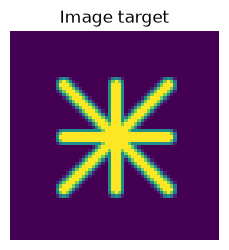
And once again, we can optimize for it.
line_init_table = {
  "rand": (
    [
      [50.89, 23.34], [44.91, 39.6], [59.01, 6.8], [28.55, 54.38],
      [42.0, 27.78], [5.16, 37.02], [4.78, 31.15], [48.51, 27.39],
      [36.28, 38.34], [3.47, 60.99], [5.04, 23.43], [4.98, 14.56],
      [38.42, 61.63], [61.46, 45.84], [20.01, 21.14], [30.59, 48.86]
    ],
    [
      [48.27, 21.45], [42.89, 41.65], [57.23, 10.7], [27.78, 65.48],
      [44.05, 34.26], [2.07, 35.97], [1.67, 33.31], [46.59, 28.99],
      [32.15, 47.97], [-2.64, 57.56], [11.03, 20.25], [9.8, 14.4],
      [44.39, 61.34], [58.65, 44.1], [20.69, 25.45], [21.08, 46.08]
    ],
    [
      1.5154, 1.1777, 0.6993, 0.8052, 1.0716, 0.6328, 0.6741, 0.3321,
      0.3307, 0.6558, 1.3163, 1.5220, 1.5364, 1.9526, 0.9107, 0.9901
    ],
  )
}
line_optimizer_table = {
  "rmsprop": (torch.optim.RMSprop, { "lr": 0.1, "momentum": 0.5 }),
  "adam": (torch.optim.Adam, { "lr": 0.5, "betas": (0.95, 0.999) }),
  "adamw": (torch.optim.AdamW, { "lr": 0.5, "betas": (0.95, 0.999) }),
}

def perform_line_run(norm_setup, optim_setup, vars_setup, steps):
  print(norm_setup, optim_setup, vars_setup, steps)
  pa_init, pb_init, rad_init = vars_setup
  p_a = nn.Parameter(torch.tensor(pa_init, dtype=torch.float32))
  p_b = nn.Parameter(torch.tensor(pb_init, dtype=torch.float32))
  p_radius = nn.Parameter(torch.tensor(rad_init))

  optim_module, optim_params = optim_setup

  optimizer = optim_module([p_a, p_b, p_radius], **optim_params)

  for step in range(steps):
    optimizer.zero_grad()
    sdf_raw = sdf_lines(grid_x, grid_y, p_a, p_b, p_radius).max(dim=-1).values
    sdf_norm = norm_setup(sdf_raw)
    loss = nn.functional.mse_loss(sdf_norm, line_target)

    loss.backward()
    optimizer.step()

    yield (step, sdf_norm.detach().clone().cpu(), line_target, loss.item())

perform_combination_test(
  perform_line_run,
  [norm_table, line_optimizer_table, line_init_table],
  ["norm_setup", "optim_setup", "vars_setup"],
  [
    dict(
      enable = True, steps = 200,
      name = "line-run-rand-adam",
      tests = [
        ("smoothstep", "adam", "rand"),
        ("atan", "adam", "rand"),
        ("atanx4", "adam", "rand"),
        ("tanh", "adam", "rand"),
        ("sigmoid", "adam", "rand"),
      ]
    ),
    dict(
      enable = True, steps = 200,
      name = "line-run-rand-adamw",
      tests = [
        ("smoothstep", "adamw", "rand"),
        ("atan", "adamw", "rand"),
        ("atanx4", "adamw", "rand"),
        ("tanh", "adamw", "rand"),
        ("sigmoid", "adamw", "rand"),
      ]
    ),
    dict(
      enable = True, steps = 200,
      name = "line-run-atanxn-adam",
      tests = [
        ("atan", "adam", "rand"),
        ("atanx1.5", "adam", "rand"),
        ("atanx2", "adam", "rand"),
        ("atanx3", "adam", "rand"),
        ("atanx4", "adam", "rand"),
      ]
    ),
  ]
)

Which gives us the following, starting with Adam:
 And then AdamW (because we haven't tested it yet):

Adam and AdamW perform nearly identically in this case. It's also interesting to note how sigmoid surprisingly manages to converge on both Adam and AdamW; it also wins basically over all other functions, maybe with the exception of atanx4.
Interestingly, smoothstep and atan fail to converge on both, so maybe atan's gradients aren't that good at all.
So now lets see how atan(xn) () performs

Only atan and atanx3 fail to converge.
Going Technicolor
Now with the optimization fundamentals out of the way, let's add color.
Adding color is quite straightforward since our sdf_lines function returns a tensor of size [W, H, M] where M is the number of lines we have.
So we can use a static canvas and basically write each shape into it by first subtracting our shape from the canvas (so we get a black void where our shape would go) and then adding it to the canvas (thus filling the void with our shape).
So this simple function is all we need:
def sdf_compose(masks, colors, bg_color):
  canvas = bg_color.expand(*masks.shape[:2], 3).clone()
  colors = colors.unsqueeze(-1).unsqueeze(-1)
  colors = colors.permute(0, 2, 3, 1)
  masks = masks.permute(2, 0, 1).unsqueeze(-1)

  for mask, color in zip(masks, colors):
    canvas = canvas * (1 - mask) + color * mask

  return canvas
Tip
Adding alpha can be done by simply pre-multiplying our mask with an alpha value.
So:
blend = mask * alpha
canvas = canvas * (1 - blend) + color * blend
With that, we achieve colored SDFs, as we can see:

Here's an animation to better visualize the whole "create shape silouette, then color and fill it" concept:
 Of course, the
 raw canvas is completely broken because we're passing the raw, non-normalized SDF values. Which is why it blends improperly.
And for completeness sake, the full code used:
def sdf_compose(masks, colors, bg_color):
  canvas = bg_color.expand(*masks.shape[:2], 3).clone()
  colors = colors.unsqueeze(-1).unsqueeze(-1)
  colors = colors.permute(0, 2, 3, 1)
  masks = masks.permute(2, 0, 1).unsqueeze(-1)

  for mask, color in zip(masks, colors):
    canvas = canvas * (1 - mask) + color * mask

  return canvas

def sdf_compose_dbg(masks, colors, bg_color):
  canvas = bg_color.expand(*masks.shape[:2], 3).clone()
  colors = colors.unsqueeze(-1).unsqueeze(-1)
  colors = colors.permute(0, 2, 3, 1)
  masks = masks.permute(2, 0, 1).unsqueeze(-1)

  intermediate_0 = []
  intermediate_1 = []
  canvas_snapshots = []

  for mask, color in zip(masks, colors):
    i_0 = canvas * (1 - mask)
    i_1 = color * mask
    canvas = i_0 + i_1
    intermediate_0.append(i_0.clone())
    intermediate_1.append(i_1.clone())
    canvas_snapshots.append(canvas.clone())

  return canvas, intermediate_0, intermediate_1, canvas_snapshots

v_a = torch.tensor([[16, 16], [16, 48], [32, 16], [16, 32]], dtype=torch.float32)
v_b = torch.tensor([[48, 48], [48, 16], [32, 48], [48, 32]], dtype=torch.float32)
v_r = torch.tensor([2, 2, 2, 2], dtype=torch.float32)
v_c = torch.tensor([[1, 0, 0], [0, 1, 0], [0, 0, 1], [1, 1, 0]], dtype=torch.float32)
v_bg = torch.tensor([0.5, 0.5, 0.5], dtype=torch.float32)

sdf_src = sdf_lines(grid_x, grid_y, v_a, v_b, v_r)
sdf_raw = sdf_compose_dbg(sdf_src, v_c, v_bg)
sdf_atan = sdf_compose_dbg(norm_atan(sdf_src), v_c, v_bg)
sdf_atanx4 = sdf_compose_dbg(norm_atanx4(sdf_src), v_c, v_bg)
sdf_tanh = sdf_compose_dbg(norm_tanh(sdf_src), v_c, v_bg)
sdf_sigmoid = sdf_compose_dbg(norm_sigmoid(sdf_src), v_c, v_bg)
sdf_smoothstep = sdf_compose_dbg(norm_smoothstep(sdf_src), v_c, v_bg)

norm_funcs = ["raw", "atan", "atanx4", "tanh", "sigmoid", "smoothstep"]
norm_list = [sdf_raw, sdf_atan, sdf_atanx4, sdf_tanh, sdf_sigmoid, sdf_smoothstep]

fig, axes = plt.subplots(1, len(norm_funcs), figsize=(16, 4))

def plot_sdf_normalizations(axes):
  for norm_idx, norm_name in enumerate(norm_funcs):
    norm_item = norm_list[norm_idx]
    plot_output(axes[norm_idx], norm_item[0], f"Lines SDF ({norm_name})", vmin=0, vmax=1)

plot_sdf_normalizations(axes)

fig.tight_layout()
plt.tight_layout()
plt.show()
plt.close()

for frame_idx in range(v_r.shape[0]):
  fig, axes = plt.subplots(3, len(norm_funcs), figsize=(16, 4 * 3))

  for norm_idx, norm_name in enumerate(norm_funcs):
    norm_item = norm_list[norm_idx]
    plot_output(axes[0, norm_idx], norm_item[1][frame_idx], f"Intermediate 0 ({norm_name})", vmin=0, vmax=1)
    plot_output(axes[1, norm_idx], norm_item[2][frame_idx], f"Intermediate 1 ({norm_name})", vmin=0, vmax=1)
    plot_output(axes[2, norm_idx], norm_item[3][frame_idx], f"Canvas ({norm_name})", vmin=0, vmax=1)

  fig.tight_layout()
  plt.tight_layout()
  plt.savefig(f"frame-{frame_idx}.png")
  plt.close()

ffmpeg_cmd = f"ffmpeg -framerate 1 -i 'frame-%d.png' -c:v libwebp -loop 0 rgb-composition-animated.webp -y"
print(subprocess.getoutput(ffmpeg_cmd))

for idx in range(v_r.shape[0]):
  os.remove(f"frame-{idx}.png")
Optimizing in color
Once again, we create a target:
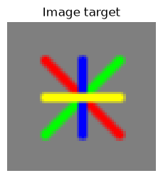
And then we optimize for it:

And again, sigmoid is the one that gets closest to convergence first. Surprisingly, most of the functions get close to convergence, but sigmoid gets there pretty fast.
You also might have noticed that it's a lot slower now; that's because I dropped the LR since the previous value was too violent for this many variables.
It's also worth noting that it uses 2 lines for the diagonal line instead of 1; while wasteful, this is a totally valid approach to optimizing this problem.
Here's how it looks when using :

Interesting how atanx1.5 and atanx2 basically fully converge.
And when using RMSprop:
 Clearly the LR is too high, but even then it does give interesting results.
Large scale demo
Now with the fundamentals out of the way, we can finally scale up to real images.
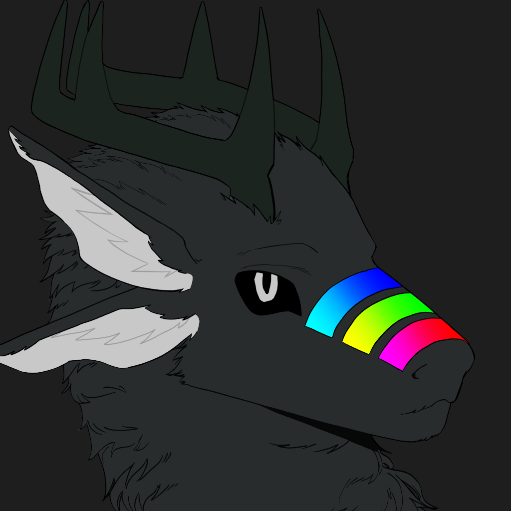
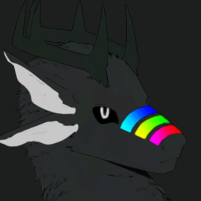
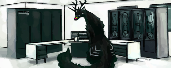
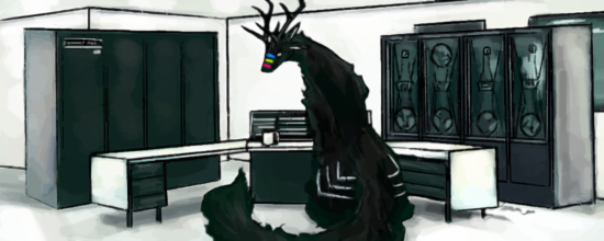
For that, I will use these images as optimization targets:
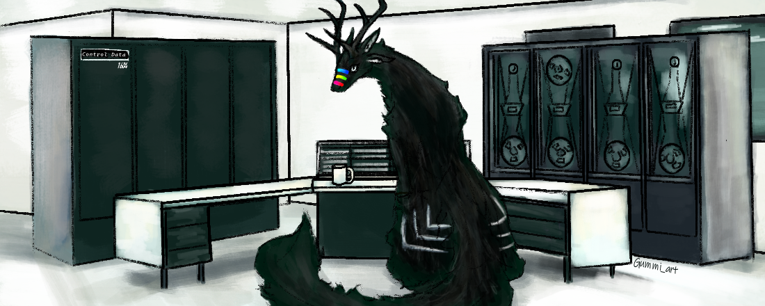
Based on what we understand now, I put together the following script:
import random
import subprocess
import sys
import time

import torch
import torchvision.transforms.functional as tv_functional
from PIL import Image, ImageDraw, ImageFont
from torch import nn, optim
from tqdm import tqdm

torch.use_deterministic_algorithms(True)
torch.manual_seed(0)
random.seed(0)

device = torch.device("cuda:0" if torch.cuda.is_available() else "cpu")
dtype = torch.float32

#"""
target_file = "optim_target_gummi_art.png"
target_res = 2

iter_count = 1500
item_count = 5000
snapshot_every = 1
#"""
"""
target_file = "optim_target_o_pastelzera_headshot.png"
target_res = 2.5

iter_count = 1500
item_count = 2000
snapshot_every = 1
#"""

image = Image.open(target_file).convert("RGB")
image = image.resize([int(sz / target_res) for sz in image.size])
image_sx, image_sy = image.size
target = tv_functional.pil_to_tensor(image).to(device, torch.float32) / 255
target_size = target.shape

x_row, y_row = [torch.arange(sz, device = device, dtype = dtype) for sz in target_size[1:]]
grid_x, grid_y = torch.meshgrid(x_row, y_row, indexing = "ij")


@torch.compile
def smoothstep(edge0: torch.Tensor | float, edge1: torch.Tensor | float, x: torch.Tensor) -> torch.Tensor:
	t = torch.clamp((x - edge0) / (edge1 - edge0 + 1e-4), 0.0, 1.0)
	return t * t * (3.0 - 2.0 * t)


# yapf: disable
@torch.compile
def norm_atanx4(sdf): return torch.atan(sdf * 4) / torch.pi + 0.5
@torch.compile
def norm_atan(sdf): return torch.atan(sdf) / torch.pi + 0.5
@torch.compile
def norm_tanh(sdf): return torch.tanh(sdf) / 2 + 0.5
@torch.compile
def norm_sigmoid(sdf): return torch.sigmoid(sdf)
@torch.compile
def norm_smoothstep(sdf): return smoothstep(-0.5, 0.5, sdf)
# yapf: enable

norm_funcs = {
	"norm_atanx4": norm_atanx4,
	"norm_atan": norm_atan,
	"norm_tanh": norm_tanh,
	"norm_sigmoid": norm_sigmoid,
	"norm_smoothstep": norm_smoothstep,
}


def init_vec_tensor(init_fn, tensor: torch.Tensor, a_list: list[float], b_list: list[float]):
	for idx, (v_a, v_b) in enumerate(zip(a_list, b_list)):
		init_fn(tensor[:, idx], v_a, v_b)


tensor_dot = torch.linalg.vecdot


@torch.compile
def tensor_length(v):
	return torch.sqrt(torch.sum(v ** 2, dim = -1) + 1e-3)


@torch.compile
def sdf_lines(grid_x: torch.Tensor, grid_y: torch.Tensor, a, b, r):
	grid = torch.cat([grid_x.unsqueeze(-1), grid_y.unsqueeze(-1)], dim = -1).unsqueeze(0)
	a = a[None, None].permute(2, 0, 1, 3)
	b = b[None, None].permute(2, 0, 1, 3)
	pa = (grid - a)
	ba = (b - a)
	h = (tensor_dot(pa, ba) / (tensor_dot(ba, ba) + 1e-3)).clamp(0, 1).unsqueeze(-1)
	return -tensor_length(pa - ba * h).permute(1, 2, 0) + r.view(1, 1, -1)


def sdf_compose(masks, colors, bg_color):
	canvas = bg_color.expand(*masks.shape[:2], 3).clone()
	canvas.to(masks.device, masks.dtype)
	colors = colors.unsqueeze(-1).unsqueeze(-1)
	colors = colors.permute(0, 2, 3, 1)
	masks = masks.permute(2, 0, 1).unsqueeze(-1)

	for mask, color in zip(masks, colors):
		canvas = canvas * (1 - mask) + color * mask

	return canvas


v_line_points_a = torch.empty(item_count, 2, requires_grad = True, dtype = dtype, device = device)
v_line_points_b = torch.empty(item_count, 2, requires_grad = True, dtype = dtype, device = device)
v_line_radius = torch.empty(item_count, requires_grad = True, dtype = dtype, device = device)
v_line_colors = torch.empty(item_count, 3, requires_grad = True, dtype = dtype, device = device)
v_color_bg = torch.empty(3, requires_grad = True, dtype = dtype, device = device)
"""
CUBLAS_WORKSPACE_CONFIG=:4096:8 &&
python optimizer_simple.py norm_atanx4 &&
python optimizer_simple.py norm_atan &&
python optimizer_simple.py norm_tanh &&
python optimizer_simple.py norm_sigmoid &&
python optimizer_simple.py norm_smoothstep
"""

norm_name = len(sys.argv) > 1 and sys.argv[1] or "norm_smoothstep"
norm_func = norm_funcs[norm_name]
output_prefix = f"out-{target_file}-{norm_name}-{int(time.time())}"

anim_info_bar_size = 40
anim_framerate = 30


def draw_items():
	masks = norm_func(sdf_lines(grid_x, grid_y, v_line_points_a, v_line_points_b, v_line_radius))
	result = sdf_compose(masks, v_line_colors, v_color_bg).permute(2, 0, 1)

	return result, masks


def pil_add_legend(
	original_image: Image.Image,
	text: str,
	bar_size: int = 40,
	bg_color = (30, 30, 30),
	fg_color = (255, 255, 255),
	font_path = None,
	font_size = 40,
):
	orig_sx, orig_sy = original_image.size

	new_sy = orig_sy + bar_size
	new_image = Image.new("RGB", (orig_sx, new_sy), color = bg_color)
	new_image.paste(original_image, (0, bar_size))

	draw = ImageDraw.Draw(new_image)

	if font_path:
		font = ImageFont.truetype(font_path, font_size)
	else:
		font = ImageFont.load_default()

	bbox = draw.textbbox((0, 0), text, font = font)
	text_sx = bbox[2] - bbox[0]

	x = (orig_sx - text_sx) // 2
	y = (bar_size - (bbox[1] + bbox[3])) // 2

	draw.text((x, y), text, fill = fg_color, font = font)

	return new_image


def clamp_params():
	with torch.no_grad():
		max_x, max_y = list(target_size[1:])
		v_line_points_a[:, 0].clamp_(0, max_x)
		v_line_points_a[:, 1].clamp_(0, max_y)
		v_line_points_b[:, 0].clamp_(0, max_x)
		v_line_points_b[:, 1].clamp_(0, max_y)
		v_line_colors.clamp_(0, 1)
		v_line_radius.clamp_(0, 16)
		v_color_bg.clamp_(0, 1)


with torch.no_grad():
	init_vec_tensor(nn.init.uniform_, v_line_points_a, [0, 0], list(target_size[1:]))
	v_line_points_b.copy_(v_line_points_a)
	v_line_points_b += torch.randn_like(v_line_points_a) * 4.0

	nn.init.uniform_(v_line_radius, 0.1, 0.2)
	init_vec_tensor(nn.init.uniform_, v_line_colors, [0, 0, 0], [1, 1, 1])
	nn.init.constant_(v_color_bg, 0.5)

clamp_params()

with torch.no_grad():
	result, masks = draw_items()
	sample = tv_functional.to_pil_image(result.detach())
	sample.save(f"{output_prefix}-init.png")

parameters = [v_line_points_a, v_line_points_b, v_line_radius, v_line_colors, v_color_bg]
optimizer = optim.Adam(parameters, lr = 0.1, betas = (0.99, 0.999), weight_decay = 0.00)

bar = tqdm(total = iter_count)

for idx in range(iter_count):
	optimizer.zero_grad()

	result, masks = draw_items()

	loss_l1 = nn.functional.l1_loss(result, target)
	loss = loss_l1
	loss.backward()

	optimizer.step()
	clamp_params()

	zero_radius = (v_line_radius <= 0).sum().item()

	if idx % snapshot_every == 0:
		with torch.no_grad():
			sample = tv_functional.to_pil_image(result.detach())
			sample = pil_add_legend(
				sample,
				f"[{idx}] {norm_name}\n"
				f"l1_loss: {loss.item():.6f}\n"
				f"v_line_radius: (zero_cnt: {zero_radius}), (mean: {v_line_radius.mean():.3f}, std: {v_line_radius.std().item():.3f})",
				bar_size = anim_info_bar_size,
			)
			sample.save(f"{output_prefix}-{idx // snapshot_every}.png")

	bar.n = idx + 1
	bar.set_postfix({
		"l": loss.item(),
		"l_l1": loss_l1.item(),
		"zero_cnt": zero_radius,
	})

with torch.no_grad():
	result, masks = draw_items()
	sample = tv_functional.to_pil_image(result.detach())
	sample.save(f"{output_prefix}-final.png")

bar.close()

with open(f"{output_prefix}-ffmpeg.txt", "w") as ffmpeg_log:
	ffmpeg_cmd = f"ffmpeg -framerate {anim_framerate} -i '{output_prefix}-%d.png' -c:v libwebp -loop 0 {output_prefix}-animated.webp -y"
	ffmpeg_out = subprocess.getoutput(ffmpeg_cmd)
	ffmpeg_log.write(ffmpeg_out)

	ffmpeg_cmd = f"ffmpeg -framerate {anim_framerate} -i '{output_prefix}-%d.png' -c:v libwebp -loop 0  -vf 'crop={image_sx}:{image_sy}:0:{anim_info_bar_size}' {output_prefix}-animated-no-bar.webp -y"
	ffmpeg_out = subprocess.getoutput(ffmpeg_cmd)
	ffmpeg_log.write(ffmpeg_out)

torch.save(
	{
		"v_line_points_a": v_line_points_a,
		"v_line_points_b": v_line_points_b,
		"v_line_radius": v_line_radius,
		"v_line_colors": v_line_colors,

		"v_color_bg": v_color_bg,
	},
	f"{output_prefix}-data.pickle",
)
And well.. It does work.

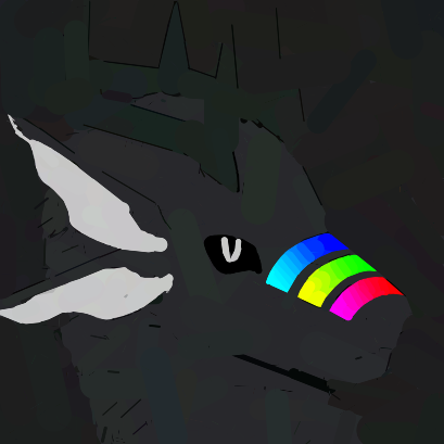

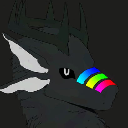
Normalization tests
So to begin with, I tested multiple normalizations.


Here are the results, from worst to best
atan:
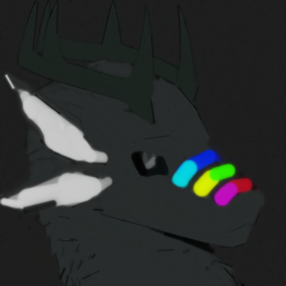

atanx4:
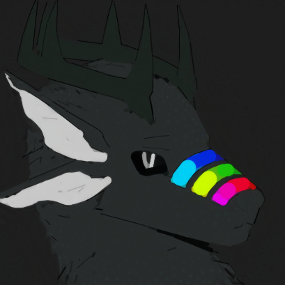
smoothstep:
tanh:

sigmoid:

From these results, we can clearly see that smoothstep, tanh, and sigmoid work the best. While atan and atanx fail very poorly at it.
Now, to me personally, it isn't 100% clear why atan and atanx fail this badly.
But I think it's somewhat safe to assume that that's because atan decays slowly, which causes the optimizer to try and optimize for "everything" at once, thus resulting in a very mediocre average.
Final results
smoothstep:
tanh:
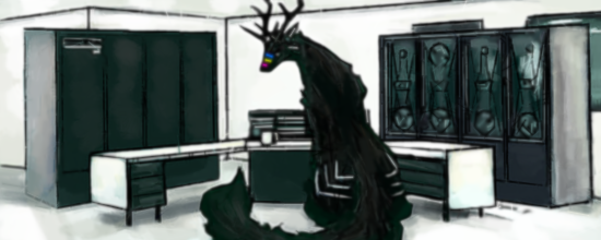
sigmoid:
Possible improvements
So... we have proven it works, and the idea is solid.
So what's next?
- We barely touched the hyperparameters, optimizers, and how initialization is performed.
We have also seen thatsigmoiddoes overall end up with better generalization, butsmoothstepgives us crisp edges. So what if we mix them both?
We could also try to optimize in multiple steps; instead of doing it in one go, we do smaller optimization runs, each one trying to decrease the difference from the target image. - It urgently needs to be optimized; we are allocating a tensor of size
WxHfor every line, no matter if that line is visible or has a radius of zero. Which, as you can imagine, isn't great when we're trying to optimize thousands of lines on larger images (a 550x220 image with 5k lines takes up basically 30GiB of VRAM, which shows its inefficiencies).
We can optimize it by splitting the area in which lines reside into 4 quadrants in the image, but this also has its own drawbacks (how will we deal with lines that go outside those quadrants?).
Another way is to perform bucketing: why allocate a hugeNxWxHtensor when we can allocate aNx16x16tensor for all primitives that use less than 16x16 of screen space?
I'm pretty sure DiffVG and similar are clever enough to pretty much not have this issue, but I haven't studied them in-depth yet, so I can't say for certain. - Doing cooler stuff.
No, but seriously, so far we just have optimized 2D images into 2D images; this same idea can be used for 3D geometry. However, that will be for a much later date.
Of course, we could solve most of these problems just by cloning DiffVG, but what's the fun in that?
I would much rather test out triton or taichi than just compiling DiffVG.
That would also mean finding out the derivatives of complex functions by hand, but that's something I will need to learn one time or another either way.
Conclusion
Well, this concludes this blog post. I believe that differentiable rendering perfectly illustrates how there really isn't a true right or wrong in ML, and that things that work great in one scenario work completely differently in another.
To give my own personal opinion about this, it isn't just about how useful differentiable rendering truly is. I think this is more about understanding and demonstrating why gradient descent is such a powerful algorithm for optimization problems.
As you can imagine, this isn't limited to just optimizing lines to raster images.
Acknowledgements
Special thanks to Exulan for providing the compute resources needed for this!
Demonstration images used courtesy of o_pastelzera and Gummi_art.